神经网络
神经网络可以通过 torch.nn 包来构建。
现在对于自动梯度(autograd)有一些了解,神经网络是基于自动梯度 (autograd)来定义一些模型。一个 nn.Module 包括层和一个方法 forward(input) 它会返回输出(output)。
例如,看一下数字图片识别的网络:
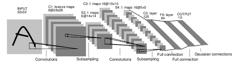
这是一个简单的前馈神经网络,它接收输入,让输入一个接着一个的通过一些层,最后给出输出。
一个典型的神经网络训练过程包括以下几点:
1.定义一个包含可训练参数的神经网络
2.迭代整个输入
3.通过神经网络处理输入
4.计算损失(loss)
5.反向传播梯度到神经网络的参数
6.更新网络的参数,典型的用一个简单的更新方法:weight = weight - learning_rate *gradient
定义神经网络
import torch
import torch.nn as nn
import torch.nn.functional as F


class Net(nn.Module):

    def __init__(self):
        super(Net, self).__init__()
        # 1 input image channel, 6 output channels, 5x5 square convolution
        # kernel
        self.conv1 = nn.Conv2d(1, 6, 5)
        self.conv2 = nn.Conv2d(6, 16, 5)
        # an affine operation: y = Wx + b
        self.fc1 = nn.Linear(16 * 5 * 5, 120)
        self.fc2 = nn.Linear(120, 84)
        self.fc3 = nn.Linear(84, 10)

    def forward(self, x):
        # Max pooling over a (2, 2) window
        x = F.max_pool2d(F.relu(self.conv1(x)), (2, 2))
        # If the size is a square you can only specify a single number
        x = F.max_pool2d(F.relu(self.conv2(x)), 2)
        x = x.view(-1, self.num_flat_features(x))
        x = F.relu(self.fc1(x))
        x = F.relu(self.fc2(x))
        x = self.fc3(x)
        return x

    def num_flat_features(self, x):
        size = x.size()[1:]  # all dimensions except the batch dimension
        num_features = 1
        for s in size:
            num_features *= s
        return num_features


net = Net()
print(net)
输出:
Net(
  (conv1): Conv2d(1, 6, kernel_size=(5, 5), stride=(1, 1))
  (conv2): Conv2d(6, 16, kernel_size=(5, 5), stride=(1, 1))
  (fc1): Linear(in_features=400, out_features=120, bias=True)
  (fc2): Linear(in_features=120, out_features=84, bias=True)
  (fc3): Linear(in_features=84, out_features=10, bias=True)
)
你刚定义了一个前馈函数,然后反向传播函数被自动通过 autograd 定义了。你可以使用任何张量操作在前馈函数上。
一个模型可训练的参数可以通过调用 net.parameters() 返回:
params = list(net.parameters())
print(len(params))
print(params[0].size())  # conv1's .weight
输出:
10
torch.Size([6, 1, 5, 5])
让我们尝试随机生成一个 32x32 的输入。注意:期望的输入维度是 32x32 。为了使用这个网络在 MNIST 数据及上,你需要把数据集中的图片维度修改为 32x32。
input = torch.randn(1, 1, 32, 32)
out = net(input)
print(out)
输出:
tensor([[-0.0233,  0.0159, -0.0249,  0.1413,  0.0663,  0.0297, -0.0940, -0.0135,
          0.1003, -0.0559]], grad_fn=<AddmmBackward>)
把所有参数梯度缓存器置零,用随机的梯度来反向传播
net.zero_grad()
out.backward(torch.randn(1, 10))
在继续之前,让我们复习一下所有见过的类。
torch.Tensor - A multi-dimensional array with support for autograd operations like backward(). Also holds the gradient w.r.t. the tensor.
nn.Module - Neural network module. Convenient way of encapsulating parameters, with helpers for moving them to GPU, exporting, loading, etc.
nn.Parameter - A kind of Tensor, that is automatically registered as a parameter when assigned as an attribute to a Module.
autograd.Function - Implements forward and backward definitions of an autograd operation. Every Tensor operation, creates at least a single Function node, that connects to functions that created a Tensor and encodes its history.
在此,我们完成了:
1.定义一个神经网络
2.处理输入以及调用反向传播
还剩下:
1.计算损失值
2.更新网络中的权重
损失函数
一个损失函数需要一对输入:模型输出和目标,然后计算一个值来评估输出距离目标有多远。
有一些不同的损失函数在 nn 包中。一个简单的损失函数就是 nn.MSELoss ,这计算了均方误差。
例如:
output = net(input)
target = torch.randn(10)  # a dummy target, for example
target = target.view(1, -1)  # make it the same shape as output
criterion = nn.MSELoss()

loss = criterion(output, target)
print(loss)
输出:
tensor(1.3389, grad_fn=<MseLossBackward>)
现在,如果你跟随损失到反向传播路径,可以使用它的 .grad_fn 属性,你将会看到一个这样的计算图:
input -> conv2d -> relu -> maxpool2d -> conv2d -> relu -> maxpool2d
      -> view -> linear -> relu -> linear -> relu -> linear
      -> MSELoss
      -> loss
所以,当我们调用 loss.backward(),整个图都会微分,而且所有的在图中的requires_grad=True 的张量将会让他们的 grad 张量累计梯度。
为了演示,我们将跟随以下步骤来反向传播。
print(loss.grad_fn)  # MSELoss
print(loss.grad_fn.next_functions[0][0])  # Linear
print(loss.grad_fn.next_functions[0][0].next_functions[0][0])  # ReLU
输出:
<MseLossBackward object at 0x7fab77615278>
<AddmmBackward object at 0x7fab77615940>
<AccumulateGrad object at 0x7fab77615940>
反向传播
为了实现反向传播损失,我们所有需要做的事情仅仅是使用 loss.backward()。你需要清空现存的梯度,要不然帝都将会和现存的梯度累计到一起。
现在我们调用 loss.backward() ,然后看一下 con1 的偏置项在反向传播之前和之后的变化。
net.zero_grad()     # zeroes the gradient buffers of all parameters

print('conv1.bias.grad before backward')
print(net.conv1.bias.grad)

loss.backward()

print('conv1.bias.grad after backward')
print(net.conv1.bias.grad)
输出:
conv1.bias.grad before backward
tensor([0., 0., 0., 0., 0., 0.])
conv1.bias.grad after backward
tensor([-0.0054,  0.0011,  0.0012,  0.0148, -0.0186,  0.0087])
现在我们看到了,如何使用损失函数。
唯一剩下的事情就是更新神经网络的参数。
更新神经网络参数:
最简单的更新规则就是随机梯度下降。
weight = weight - learning_rate * gradient
我们可以使用 python 来实现这个规则:
learning_rate = 0.01
for f in net.parameters():
    f.data.sub_(f.grad.data * learning_rate)
尽管如此,如果你是用神经网络,你想使用不同的更新规则,类似于 SGD, Nesterov-SGD, Adam, RMSProp, 等。为了让这可行,我们建立了一个小包:torch.optim 实现了所有的方法。使用它非常的简单。
import torch.optim as optim

# create your optimizer
optimizer = optim.SGD(net.parameters(), lr=0.01)

# in your training loop:
optimizer.zero_grad()   # zero the gradient buffers
output = net(input)
loss = criterion(output, target)
loss.backward()
optimizer.step()    # Does the update
下载 Python 源代码:
下载 Jupyter 源代码: